The goal of the muscle force model is to simulate the behavior of a muscle as a function of its length and innervation. This is achieved by the definition of three force functions (contractile, elastic and total force). In order to modify the behavior of a muscle for e.g. simulating muscle palsies (paresis) or hyperfunctions, the force model offers several different parameters, which change the shape of the simulation curves in certain ways in order to simulate the desired situation.

 

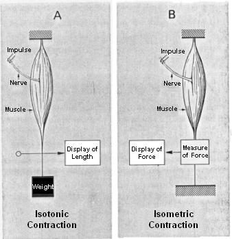
During the examination of muscle forces, one differentiates two types of muscle contraction: isotonic contraction and isometric contraction. An isotonic contraction is used for the measurement of the muscle length and length change due to an activation with constant load (see figure A). In case of the isometric contraction, the strength and the change of force of the muscle is measured with the length held constant (see figure B). The contraction mechanism takes place on molecular level and is described by the so-called filament sliding theory. Actin and myosin filaments are connected by so-called bridges and allow an activation-triggered shortening and thus the development of muscle strength.

 

Different Types of Muscle Contraction Measurement

 

In general, static and dynamic characteristics of a muscle can be differentiated. Static force behavior is also called force-length relationship. As a starting point, an isometric force measurement is carried out and the measured force is recorded depending on the previously set (fixed) length. Dynamic characteristics of a muscle refer to contraction speeds and are analyzed by isotonic measurements. SEE++ currently represents only a static model of muscle force development and concentrates on the modeling of force-length-innervation relationships.

In the representation of static characteristics of a muscle, one differentiates again between contractile (active) and elastic (passive) muscle forces. Contractile muscle forces result from activation (innervation) of a muscle by the brain, while elastic forces represent the elastic stretch-characteristics of a muscle, which work opposite to the contractile forces. By applying repeated isometric force measurements with differently adjusted lengths, a force-length curve of the muscle behavior results. In relating these data to the activation potential of a muscle, a three-dimensional force-length-activation function is the result. This function again can be divided into its contractile and elastic forces receiving a contractile and elastic force curve, which together correspond to the total force curve of a muscle.

The elastic force curve describes the elastic forces, which the muscle exerts when it is stretched or compressed accordingly. If a detached muscle is sufficiently stretched, then, at a certain length, this muscle won't behave like a non-linear spring anymore, but will get stiff very fast, allowing no further stretching. This is called "leash-region" and becomes apparent in a drastic rise of the passive strength with increased stretch length. On the contrary, if a muscle is strongly pushed together in its length (shortened), then it will get slack and cannot exert force anymore. This is called the "slack-region" of the muscle force function.

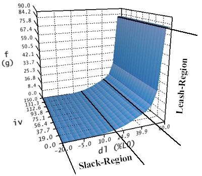
Elastic Force-Length Curve

 

Like shown in the figure, the elastic force-length curve does not depend on the activation (iv) of a muscle, since only passive, elastic forces are modelled. This is also the reason why, for all innervations, the curve has the same shape in the length-innervation-plane. The elastic force curve is calculated in three intervals (dl < 17%; 17% <= dl <= 40%; dl > 40%) referring to the axis of the muscle's length. The unit used for this axis is the length change in percent referring to the relaxed, denervated length of the muscle (L0). In the first region (dl < 17%) the muscle force has been changed by hand to converge against zero, while in the third region (dl > 40%) the force was extrapolated up to a specific maximum in order to simulate the rapid increase of the stiffness of the muscle in the "leash-region". Between the first and the third region (17% <= dl <= 40%) the elasticity is calculated with a non-linear spring equation.

The contractile force curve now describes the resulting contractile force in dependence of innervation and length of a muscle.

 

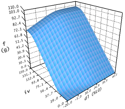
Contractile Force Curve

 

This curve is also divided into three regions. The first region is calculated within the interval -20% <= dl <= 45% and 0 <= iv <= 100. The second region in the area of -20% <= dl <= 45% and iv > 100 is calculated by extrapolating the values from the first interval. The third region for dl > 45% is constantly calculated like dl = 45%.

The total force function is now calculated as the sum of the elastic and contractile force function.

 

In order to change the behavior of the extraocular muscles within the force model of SEE++, the system offers a number of parameters, which allow to manipulate the different curves. Three global parameters are available which influence all six muscles and specify the shape of the curves in the transition region between slack and leash region.

 

•Stiffness (g/% á L0) defines the rise of the curve towards the leash region, in order to approximate the overexpansion behaviour of the musculature. The unit therefore is gram per percent on the basis of the relaxed muscle length (L0). This value should only be changed in a very small range of 0 <= x <= 0.9.

•Force transition scaling (g) defines the shape of the curve at the transition to the slack region. The unit for this value is gram and it describes how much the curve is damped in the rising area of the calculated (second) interval. The smaller this value is, the longer the force is zero when the muscle is stretched. This also corresponds to a punctual expansion of the slack region.

•Force displacement ratio (% á L0) shifts the calculated (second) region of each curve on the axis of the muscle's length-change (dl). The displacement is specified in percent of the relaxed muscle length (L0).

 

Basically, the described parameters should only be used for experimenting with the force model of SEE++. These values should only be changed with the utmost care, because these changes strongly influence the simulation result.

 

Muscle-Specific Parameters

In the SEE++ system all six eye muscles are simulated with the described force model. The difference in the force development of each muscle is defined by two scaling factors (one for the elastic and one for the contractile force), which modify the force curves in relation to the lateral rectus muscle. The following parameters are available for each muscle:

 

•Elastic strength (%/100) scales the elastic force curve in order to influence the elastic properties of a muscle. A reduction of this value, for example, results in a muscle with a reduced elastic force when the muscle stretches.

•Contractile strength (%/100) scales the contractile force curve and simulates a hyperfunction or a muscle palsy in relation to the cerebral activation. A value of zero would correspond to a complete muscle paresis (complete loss of the contractile strength).

•Relative elastic strength (%/100 RL) scales the elastic force function with respect to the lateral rectus muscle. If this values is changed, a muscle is strengthened or weakened relative to the lateral rectus muscle; in order to modify the elastic strength relative to the current muscle, the parameter "elastic strength" should be directly used.

•Relative contractile strength (%/100 RL) scales the contractile force function with respect to the lateral rectus muscle. If this value is changed, a muscle is strengthened or weakened relative to the lateral rectus muscle; in order to modify the contractile strength relative to the current muscle, the parameter "contractile strength" should be directly used.

 

For the simulation of surgeries, the length of a muscle is also very important. The length of the muscle and the tendon also changes the way how the simulation system "interprets" the muscle force curves. The modification of muscle length (dl) is shown in percent in the muscle force curves. As an example, a rubber band with a length of 10 mm is used (relaxed length L0=10 mm). If this rubber band is stretched by 10 mm, one receives a path length of 20 mm and a relative stretch of 100%. If the band is now shortened to 5 mm relaxed length and once again the band is stretched by 10 mm, a relative stretch of 200% results. This would lead to a totally different resulting force in the force model and shows, how the modification of muscle length can influence the force behaviour of a muscle.

 

The muscle model of SEE++ offers the following parameters:

 

•Muscle length (L0) in mm specifies the length of a relaxed, denervated muscle without the tendon.

•Tendon length in mm specifies the additional length of the tendon.

•Tendon width in mm specifies the width of the tendon at the insertion and is used for the distribution of force over the muscle's width.

 

For example, to simulate a resection of the lateral rectus muscle by 5 mm, the length of the muscle and/or the tendon has to be changed accordingly. When the insertion of the lateral rectus muscle is separated from the globe, the muscle is shortened by 5 mm and afterwards the muscle is fixed again at the same position, one usually loses 1 mm of the length of the muscle and/or the tendon during the separation and 1 mm during the re-fixation (due to different surgery techniques, these values can vary and have to be corrected individually). Since SEE++ cannot consider these circumstances automatically, it is necessary to shorten the muscle by 7 mm in this situation. Therefore, the tendon length of lateral rectus muscle would be changed from 7.71 mm to 0.71 mm. If a larger resection is carried out, it is possible that the muscle loses its tendon (tendon length = 0) and in such a case the remaining shortening has to be applied to the muscle length, consequently both parameters have to be changed. With the help of the surgery method "Resection", which can be carried out in the "Non-Graphical Surgery" dialog, this reduction of the tendon length to 0 mm and the following reduction of the muscle length during a larger resection are made automatically.

 

Another parameter, which is only used in the Orbit force model, is the pulley stiffness. With this parameter, the passive movement of a pulley is limited in g/mm. Changes to this parameter and, as a consequence, the movement of the pulley in different gaze positions, affect the direction of pull of a muscle and transitively affect the muscle's force behaviour.

 

Innervation of Eye Muscles

The eye muscles are innervated by three cranial nerves. The nervus oculomotorius (III. cranial nerve) innervates the medial rectus muscle, the superior rectus muscle, the inferior rectus muscle and the inferior oblique muscle (moreover the levator palpebrae as well as - with its parasympathetic part - the ciliaris muscle and the sphincter pupillae muscle). The nervus trochlearis (IV. cranial nerve) innervates the superior oblique muscle and the nervus abducens (VI. cranial nerve) innervates the lateral rectus muscle. Each eye muscle is innervated by approximately 1000 motoneurons. The single motoneurons branch out into the eye muscle and innervate approximately 4 to 40 muscle fibers at a time. A motor unit is the aggregation of those muscle fibers, which are connected to one and the same motoneuron.

 

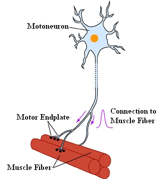
A Motor Unit of a Muscle Consists of a

Motoneuron with All Muscle Fibers Innervated by This Neuron

 

The brain uses two different possibilities to increase the traction force of a muscle:

 

Motor Nuclei

The cell bodies of the motoneurons lie together in pairs and form the so-called nuclei within the brainstem. The nuclei area of the two oculomotoric nerves lies inside the midbrain. The alignment of those parts of the nuclei, which are associated with the specific eye muscles, is very complicated and most of the details have been examined as recently as in the last few years. The cell bodies of the medial rectus muscle, the inferior rectus muscle and the inferior oblique muscle lie ipsilaterally (i.e. for the right eye on the right nucleus-side). Only the cell bodies of the superior rectus muscle lie contralaterally (i.e. for the right eye on the left side of the III. nucleus pair). The nerve fibers of the superior rectus muscle cross in the area of the oculomoter nuclei to the other side. The cell bodies of the levator palpebrae muscle lie close to the middle line, both ipsilateral and contralateral.

The two nuclei of the nervus trochlearis also lie in the midbrain just below the area of the oculomotor nuclei. The motoneurons of the nervus trochlearis originate contralaterally and cross behind the aqueduct, below the lamina quadrigemina, to the other side.

The nuclei of the nervus abducens lie in the bridge and are linked to the respective ipsilateral lateral rectus muscle.

 

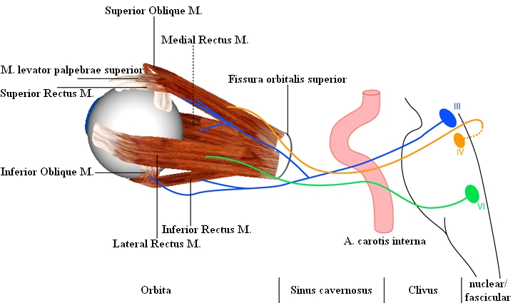
Location of the Oculomotor Nuclei and Course of the Oculomotor Cranial Nerves

 

The SEE++ system does not contain its own simulation of the brainstem or the supranuclear structures. However, it realizes a so-called distribution of innervations for each eye, which makes it possible to change the percentage of innervation distributed from the oculomotor nuclei to the respective muscles. If such a distribution is modified, all innervations in relation to the affected muscle of the affected eye are scaled in percent.

 

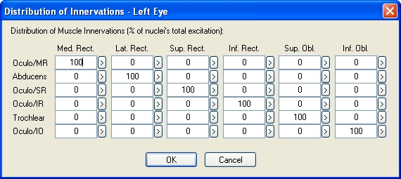
Example of the Distribution of Innervations of the Left Eye (Based on Orbit™, See [Miller, 1999])

 

By modifying the distribution of innervations, it is possible to simulate either internuclear or supranuclear gaze palsies as well as, for example, retraction syndromes. A supranuclear gaze palsy when looking to the right would be simulated by changing the distribution of innervations of the nervus abducens to the lateral rectus muscle on the right eye and by changing the distribution of the nervus oculomotorius to the medial rectus muscle on the left eye. During a "simple" internuclear gaze palsy only one eye would be affected (saccades) and therefore only the distribution of innervations of one eye would require changes.

 

SEE++ uses a so-called invisible reference eye, which is used as basis for the calculations. If the distribution of innervations of this reference eye is changed, only the reciprocal following eye would reflect these changes in the Hess-Lancaster test. This allows for example the simulation of a lesion, which is only visible when observing the following eye.